Compute the scattering transform of a synthetic signal

In this example we generate a harmonic signal of a few different frequencies and analyze it with the 1D scattering transform.

Import the necessary packages

from kymatio.numpy import Scattering1D
import matplotlib.pyplot as plt
import numpy as np

Write a function that can generate a harmonic signal

Let’s write a function that can generate some simple blip-type sounds with decaying harmonics. It will take four arguments: T, the length of the output vector; num_intervals, the number of different blips; gamma, the exponential decay factor of the harmonic; random_state, a random seed to generate random pitches and phase shifts. The function proceeds by splitting the time length T into intervals, chooses base frequencies and phases, generates sinusoidal sounds and harmonics, and then adds a windowed version to the output signal.

def generate_harmonic_signal(T, num_intervals=4, gamma=0.9, random_state=42):
    """
    Generates a harmonic signal, which is made of piecewise constant notes
    (of random fundamental frequency), with half overlap
    """
    rng = np.random.RandomState(random_state)
    num_notes = 2 * (num_intervals - 1) + 1
    support = T // num_intervals
    half_support = support // 2

    base_freq = 0.1 * rng.rand(num_notes) + 0.05
    phase = 2 * np.pi * rng.rand(num_notes)
    window = np.hanning(support)
    x = np.zeros(T, dtype='float32')
    t = np.arange(0, support)
    u = 2 * np.pi * t
    for i in range(num_notes):
        ind_start = i * half_support
        note = np.zeros(support)
        for k in range(1):
            note += (np.power(gamma, k) *
                     np.cos(u * (k + 1) * base_freq[i] + phase[i]))
        x[ind_start:ind_start + support] += note * window

    return x

Let’s take a look at what such a signal could look like

T = 2 ** 13
x = generate_harmonic_signal(T)
plt.figure(figsize=(8, 2))
plt.plot(x)
plt.title("Original signal")

Text(0.5, 1.0, 'Original signal')

Spectrogram

Let’s take a look at the signal spectrogram

plt.figure(figsize=(8, 4))
plt.specgram(x, Fs=1024)
plt.title("Time-Frequency spectrogram of signal")

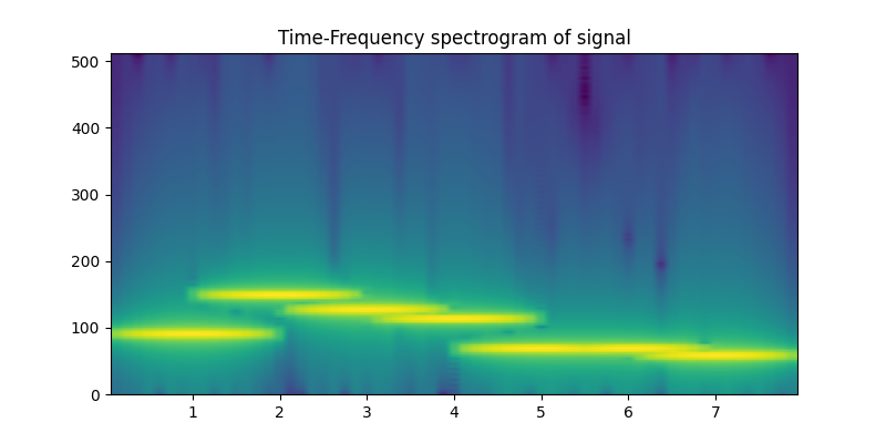
Text(0.5, 1.0, 'Time-Frequency spectrogram of signal')

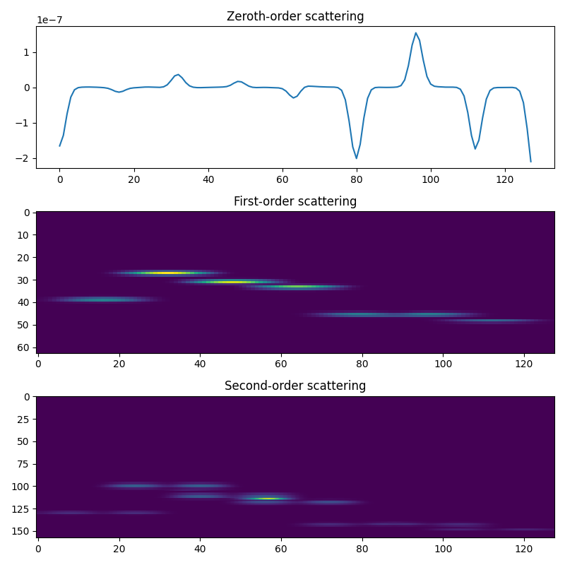
Doing the scattering transform

J = 6
Q = 16

scattering = Scattering1D(J, T, Q)

meta = scattering.meta()
order0 = np.where(meta['order'] == 0)
order1 = np.where(meta['order'] == 1)
order2 = np.where(meta['order'] == 2)

Sx = scattering(x)

plt.figure(figsize=(8, 8))
plt.subplot(3, 1, 1)
plt.plot(Sx[order0][0])
plt.title('Zeroth-order scattering')
plt.subplot(3, 1, 2)
plt.imshow(Sx[order1], aspect='auto')
plt.title('First-order scattering')
plt.subplot(3, 1, 3)
plt.imshow(Sx[order2], aspect='auto')
plt.title('Second-order scattering')
plt.tight_layout()
plt.show()