User guide

Introduction to scattering transforms

A scattering transform is a non-linear signal representation that builds invariance to geometric transformations while preserving a high degree of discriminability. These transforms can be made invariant to translations, rotations (for 2D or 3D signals), frequency shifting (for 1D signals), or changes of scale. These transformations are often irrelevant to many classification and regression tasks, so representing signals using their scattering transform reduces unnecessary variability while capturing structure needed for a given task. This reduced variability simplifies the building of models, especially given small training sets.

The scattering transform is defined as a complex-valued convolutional neural network whose filters are fixed to be wavelets and the non-linearity is a complex modulus. Each layer is a wavelet transform, which separates the scales of the incoming signal. The wavelet transform is contractive, and so is the complex modulus, so the whole network is contractive. The result is a reduction of variance and a stability to additive noise. The separation of scales by wavelets also enables stability to deformation of the original signal. These properties make the scattering transform well-suited for representing structured signals such as natural images, textures, audio recordings, biomedical signals, or molecular density functions.

Let us consider a set of wavelets \(\{\psi_\lambda\}_\lambda\), such that there exists some \(\epsilon\) satisfying:

\[1-\epsilon \leq \sum_\lambda |\hat \psi_\lambda(\omega)|^2 \leq 1\]

Given a signal \(x\), we define its scattering coefficient of order \(k\) corresponding to the sequence of frequencies \((\lambda_1,...,\lambda_k)\) to be

\[Sx[\lambda_1,...,\lambda_k] = |\psi_{\lambda_k} \star ...| \psi_{\lambda_1} \star x|...|\]

For a general treatment of the scattering transform, see [Mal12]. More specific descriptions of the scattering transform are found in [AndenM14] for 1D, [BM13] for 2D, and [EEHM17] for 3D.

Practical implementation

Previous implementations, such as ScatNet [AndenSM+14], of the scattering transform relied on computing the scattering coefficients layer by layer. In Kymatio, we instead traverse the scattering transform tree in a depth-first fashion. This limits memory usage and makes the implementation better suited for execution on a GPU. The difference between the two approaches is illustrated in the figure below.

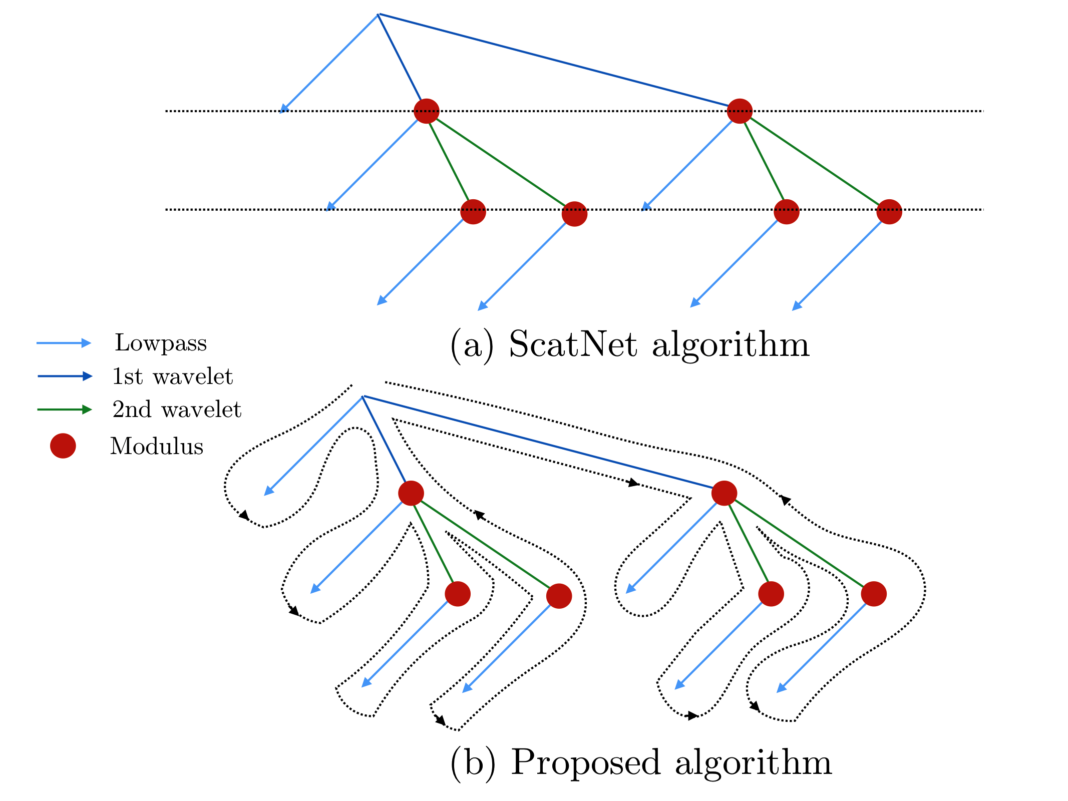
The scattering tree traversal strategies of (a) the ScatNet toolbox, and (b) Kymatio. While ScatNet traverses the tree in a breadth-first fashion (layer by layer), Kymatio performs a depth-first traversal.

More details about our implementation can be found in Information for developers.

1-D

The 1D scattering coefficients computed by Kymatio are similar to those of ScatNet [AndenSM+14], but do not coincide exactly. This is due to a slightly different choice of filters, subsampling rules, and coefficient selection criteria. The resulting coefficients, however, have a comparable performance for classification and regression tasks.

2-D

The 2D implementation in this package provides scattering coefficients that exactly match those of ScatNet [AndenSM+14].

3-D

The 3D scattering transform is currently limited to solid harmonic wavelets, which are solid harmonics (spherical harmonics multiplied by a radial polynomial) multiplied by Gaussians of different width. They perform scale separation and feature extraction relevant to e.g. molecule structure while remaining perfectly covariant to transformations with the Euclidean group.

The current implementation is very similar to the one used in [EEHM17], and while it doesn’t correspond exactly, it makes use of better theory on sampling and leads to similar performance on QM7.

Output size

1-D

If the input \(x\) is a Tensor of size \((B, T)\), the output of the 1D scattering transform is of size \((B, P, T/2^J)\), where \(P\) is the number of scattering coefficients and \(2^J\) is the maximum scale of the transform. The value of \(P\) depends on the maximum order of the scattering transform and the parameters \(Q\) and \(J\). It is roughly proportional to \(1 + J Q + J (J-1) Q / 2\).

2-D

Let us assume that \(x\) is a tensor of size \((B,C,N_1,N_2)\). Then the output \(Sx\) via a Scattering Transform with scale \(J\) and \(L\) angles and \(m\) order 2 will have size:

\[(B,C,1+LJ+\frac{L^2J(J-1)}{2},\frac{N_1}{2^J},\frac{N_2}{2^J})\]

3-D

For an input array of shape \((B, C, N_1, N_2, N_3)\), a solid harmonic scattering with \(J\) scales and \(L\) angular frequencies, which applies \(P\) different types of \(\mathcal L_p\) spatial averaging, and \(m\) order 2 will result in an output of shape

\[(B, C, 1+J+\frac{J(J + 1)}{2}, 1+L, P)\,.\]

The current configuration of Solid Harmonic Scattering reflects the one in [EEHM17] in that second order coefficients are obtained for the same angular frequency only (as opposed to the cartesian product of all angular frequency pairs), at higher scale.

Frontends

The Kymatio API is divided between different frontends, which perform the same operations, but integrate in different frameworks. This integration allows the user to take advantage of different features available in certain frameworks, such as autodifferentiation and GPU processing in PyTorch and TensorFlow/Keras, while having code that runs almost identically in NumPy or scikit-learn. The available frontends are:

• kymatio.numpy for NumPy,

• kymatio.sklearn for scikit-learn (as Transformer and Estimator objects),

• kymatio.torch for PyTorch,

• kymatio.tensorflow for TensorFlow, and

• kymatio.keras for Keras.

To instantiate a Scattering2D object for the numpy frontend, run:

from kymatio.numpy import Scattering2D
S = Scattering2D(J=2, shape=(32, 32))

Alternatively, the object may be instantiated in a dynamic way using the kymatio.Scattering2D object by providing a frontend argument. This object then transforms itself to the desired frontend. Using this approach, the above example becomes:

from kymatio import Scattering2D
S = Scattering2D(J=2, shape=(32, 32), frontend='numpy')

In Kymatio 0.2, the default frontend is torch for backwards compatibility reasons, but this change to numpy in the next version.

NumPy

The NumPy frontend takes ndarrays as input and outputs ndarrays. All computation is done on the CPU, which means that it will be slow for large inputs. To call this frontend, run:

from kymatio.numpy import Scattering2D

scattering = Scattering2D(J=2, shape=(32, 32))

This will only use standard NumPy routines to calculate the scattering transform.

Scikit-learn

For scikit-learn, we have the sklearn frontend, which is both a Transformer and an Estimator, making it easy to integrate the object into a scikit-learn Pipeline. For example, you can write the following:

from sklearn.pipeline import Pipeline
from sklearn.linear_model import LogisticRegression

from kymatio.sklearn import Scattering2D

S = Scattering2D(J=1, shape=(8, 8))
classifier = LogisticRegression()
pipeline = Pipeline([('scatter', S), ('clf', classifier)])

which creates a Pipeline consisting of a 2D scattering transform and a logistic regression estimator.

PyTorch

If PyTorch is installed, we may also use the torch frontend, which is implemented as a torch.nn.Module. As a result, it can be integrated with other PyTorch Modules to create a computational model. It also supports the cuda(), cpu(), and to() methods, allowing the user to easily move the object from CPU to GPU and back. When initialized, a scattering transform object is stored on the CPU:

from kymatio.torch import Scattering2D

scattering = Scattering2D(J=2, shape=(32, 32))

We use this to compute scattering transforms of signals in CPU memory:

import torch
x = torch.randn(1, 1, 32, 32)

Sx = scattering(x)

If a CUDA-enabled GPU is available, we may transfer the scattering transform object to GPU memory by calling cuda():

scattering.cuda()

Transferring the signal to GPU memory as well, we can then compute its scattering coefficients:

x_gpu = x.cuda()
Sx_gpu = scattering(x)

Transferring the output back to CPU memory, we may then compare the outputs:

Sx_gpu = Sx_gpu.cpu()
print(torch.norm(Sx_gpu-Sx))

These coefficients should agree up to machine precision. We may transfer the scattering transform object back to the CPU by calling cpu(), like this:

scattering.cpu()

TensorFlow

If TensorFlow is installed, you may use the tensorflow frontend, which is implemented as a tf.Module. To call this frontend, run:

from kymatio.tensorflow import Scattering2D
scattering = Scattering2D(J=2, shape=(32, 32))

This is a TensorFlow module that one can use directly in eager mode. Like other modules (and like the torch frontend), you may transfer it onto and off the GPU using the cuda() and cpu() methods.

Keras

For compatibility with the Keras framework, we also include a keras frontend, which wraps the TensorFlow class in a Keras Layer, allowing us to include it in a Model with relative ease. Note that since Keras infers the input shape of a Layer, we do not specify the shape when creating the scattering object. The result may look something like:

from tensorflow.keras.models import Model
from tensorflow.keras.layers import Input, Flatten, Dense

from kymatio.keras import Scattering2D

in_layer = Input(shape=(28, 28))
sc = Scattering2D(J=3)(in_layer)
sc_flat = Flatten()(sc)
out_layer = Dense(10, activation='softmax')(sc_flat)

model = Model(in_layer, out_layer)

where we feed the scattering coefficients into a dense layer with ten outputs for handwritten digit classification on MNIST.

Backend

The backends encapsulate the most computationally intensive part of the scattering transform calculation. As a result, improved performance can often be achieved by replacing the default backend with a more optimized alternative.

For instance, the default backend of the torch frontend is the torch backend, implemented exclusively in PyTorch. This is available for 1D, 2D, and 3D. It is also compatible with the PyTorch automatic differentiation framework, and runs on both CPU and GPU. If one wants additional improved performance on GPU, we recommended to use the torch_skcuda backend.

Currently, two backends exist for torch:

• torch: A PyTorch-only implementation which is differentiable with respect to its inputs. However, it relies on general-purpose CUDA kernels for GPU computation which reduces performance.

• torch17: Same as above, except it is compatible with the version <=1.7.1 of PyTorch.

• torch_skcuda: An implementation using custom CUDA kernels (through cupy) and scikit-cuda. This implementation only runs on the GPU (that is, you must call cuda() prior to applying it). Since it uses kernels optimized for the various steps of the scattering transform, it achieves better performance compared to the default torch backend (see benchmarks below). This improvement is currently small in 1D and 3D, but work is underway to further optimize this backend.

• torch17_skcuda: Same as above, except it is compatible with the version <=1.7.1 of PyTorch.

This backend can be specified via:

import torch
from kymatio.torch import Scattering2D

scattering = Scattering2D(J=2, shape=(32, 32), backend='torch_skcuda')

Each of the other frontends currently only has a single backend, which is the default. Work is currently underway, however, to extend some of these frontends with more powerful backends.

Benchmarks

1D

We compared our implementation with that of the ScatNet MATLAB package [AndenSM+14] with similar settings. The following table shows the average computation time for a batch of size \(64 \times 65536\). This corresponds to \(64\) signals containing \(65536\), or a total of about \(95\) seconds of audio sampled at \(44.1~\mathrm{kHz}\).

Name	Average time per batch (s)
ScatNet [AndenSM+14]	1.65
Kymatio (torch frontend-backend, CPU)	2.74
Kymatio (torch frontend-backend, Quadro M4000 GPU)	0.81
Kymatio (torch frontend-backend, V100 GPU) 0.15
Kymatio (torch frontend, skcuda backend, Quadro M4000 GPU)	0.66
Kymatio (torch frontend, skcuda backend, V100 GPU)	0.11

The CPU tests were performed on a 24-core machine. Further optimization of both the torch and skcuda backends is currently underway, so we expect these numbers to improve in the near future.

2D

We compared our implementation the ScatNetLight MATLAB package [OM15] and a previous PyTorch implementation, PyScatWave [OZH+18]. The following table shows the average computation time for a batch of size \(128 \times 3 \times 256 \times 256\). This corresponds to \(128\) three-channel (e.g., RGB) images of size \(256 \times 256\).

Name	Average time per batch (s)
MATLAB [OM15]	>200
Kymatio (torch frontend-backend, CPU)	110
Kymatio (torch frontend-backend, 1080Ti GPU)	4.4
Kymatio (torch frontend-backend, V100 GPU)	2.9
PyScatWave (1080Ti GPU)	0.5
Kymatio (torch frontend, skcuda backend, 1080Ti GPU)	0.5

The CPU tests were performed on a 48-core machine.

3D

We compared our implementation for different backends with a batch size of \(8 \times 128 \times 128 \times 128\). This means that eight different volumes of size \(128 \times 128 \times 128\) were processed at the same time. The resulting timings are:

Name	Average time per batch (s)
Kymatio (torch frontend-backend, CPU)	45
Kymatio (torch frontend-backend, Quadro M4000 GPU)	7.5
Kymatio (torch frontend-backend, V100 GPU)	0.88
Kymatio (torch frontend, skcuda backend, Quadro M4000 GPU)	6.4
Kymatio (torch frontend, skcuda backend, V100 GPU)	0.74

The CPU tests were performed on a 24-core machine. Further optimization of both the torch and skcuda backends is currently underway, so we expect these numbers to improve in the near future.

How to cite

If you use this package, please cite the following paper:

Andreux M., Angles T., Exarchakis G., Leonarduzzi R., Rochette G., Thiry L., Zarka J., Mallat S., Andén J., Belilovsky E., Bruna J., Lostanlen V., Hirn M. J., Oyallon E., Zhang S., Cella C., Eickenberg M. (2019). Kymatio: Scattering Transforms in Python. arXiv preprint arXiv:1812.11214. (paper)

References

[AndenM14]

J. Andén and S. Mallat. Deep scattering spectrum. IEEE Trans. Signal Process., 62:4114–4128, 2014.

[AndenSM+14] (1,2,3,4,5)

J Andén, L Sifre, S Mallat, M Kapoko, V Lostanlen, and E Oyallon. Scatnet. Computer Software. Available: http://www.di.ens.fr/data/software/scatnet, 2014.

[BM13]

J. Bruna and S. Mallat. Invariant scattering convolution networks. IEEE Trans. Pattern Anal. Mach. Intell., 35(8):1872–1886, 2013.

[EEHM17] (1,2,3)

Michael Eickenberg, Georgios Exarchakis, Matthew Hirn, and Stéphane Mallat. Solid harmonic wavelet scattering: predicting quantum molecular energy from invariant descriptors of 3d electronic densities. In Advances in Neural Information Processing Systems, 6540–6549. 2017.

[Mal12]

Stéphane Mallat. Group invariant scattering. Communications on Pure and Applied Mathematics, 65(10):1331–1398, 2012.

[OZH+18]

E. Oyallon, S. Zagoruyko, G. Huang, N. Komodakis, S. Lacoste-Julien, M. B. Blaschko, and E. Belilovsky. Scattering networks for hybrid representation learning. IEEE Transactions on Pattern Analysis and Machine Intelligence, ():1–1, 2018. doi:10.1109/TPAMI.2018.2855738.

[OM15] (1,2)

Edouard Oyallon and Stephane Mallat. Deep roto-translation scattering for object classification. In The IEEE Conference on Computer Vision and Pattern Recognition (CVPR). June 2015.