Compute the scattering transform of a speech recording

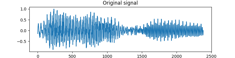
This script loads a speech signal from the free spoken digit dataset (FSDD) of a man pronouncing the word “zero,” computes its scattering transform, and displays the zeroth-, first-, and second-order scattering coefficients.

Preliminaries

import numpy as np
import os
import scipy.io.wavfile

We import matplotlib to plot the calculated scattering coefficients.

import matplotlib.pyplot as plt

Finally, we import the Scattering1D class from the scattering package and the fetch_fsdd function from scattering.datasets. The Scattering1D class is what lets us calculate the scattering transform, while the fetch_fsdd function downloads the FSDD, if needed.

from kymatio.numpy import Scattering1D
from kymatio.datasets import fetch_fsdd

Scattering setup

First, we download the FSDD (if not already downloaded) and read in the recording 0_jackson_0.wav of a man pronouncing the word “zero”.

info_dataset = fetch_fsdd(verbose=True)

file_path = os.path.join(info_dataset['path_dataset'], sorted(info_dataset['files'])[0])
_, x = scipy.io.wavfile.read(file_path)

Cloning git repository at  https://github.com/Jakobovski/free-spoken-digit-dataset.git

Once the recording is in memory, we normalize it.

x = x / np.max(np.abs(x))

We are now ready to set up the parameters for the scattering transform. First, the number of samples, T, is given by the size of our input x. The averaging scale is specified as a power of two, 2**J. Here, we set J = 6 to get an averaging, or maximum, scattering scale of 2**6 = 64 samples. Finally, we set the number of wavelets per octave, Q, to 16. This lets us resolve frequencies at a resolution of 1/16 octaves.

T = x.shape[-1]
J = 6
Q = 16

Finally, we are able to create the object which computes our scattering transform, scattering.

scattering = Scattering1D(J, T, Q)

Compute and display the scattering coefficients

Computing the scattering transform of a signal is achieved using the __call__ method of the Scattering1D class. The output is an array of shape (C, T). Here, C is the number of scattering coefficient outputs, and T is the number of samples along the time axis. This is typically much smaller than the number of input samples since the scattering transform performs an average in time and subsamples the result to save memory.

Sx = scattering(x)

To display the scattering coefficients, we must first identify which belong to each order (zeroth, first, or second). We do this by extracting the meta information from the scattering object and constructing masks for each order.

meta = scattering.meta()
order0 = np.where(meta['order'] == 0)
order1 = np.where(meta['order'] == 1)
order2 = np.where(meta['order'] == 2)

First, we plot the original signal x.

plt.figure(figsize=(8, 2))
plt.plot(x)
plt.title('Original signal')

Text(0.5, 1.0, 'Original signal')

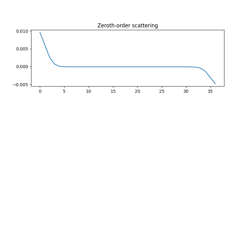
We now plot the zeroth-order scattering coefficient, which is simply an average of the original signal at the scale 2**J.

plt.figure(figsize=(8, 8))
plt.subplot(3, 1, 1)
plt.plot(Sx[order0][0])
plt.title('Zeroth-order scattering')

Text(0.5, 1.0, 'Zeroth-order scattering')

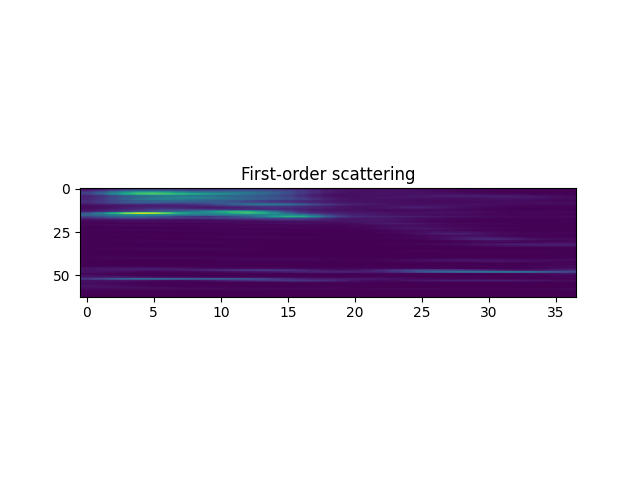
We then plot the first-order coefficients, which are arranged along time and log-frequency.

plt.subplot(3, 1, 2)
plt.imshow(Sx[order1], aspect='auto')
plt.title('First-order scattering')

Text(0.5, 1.0, 'First-order scattering')

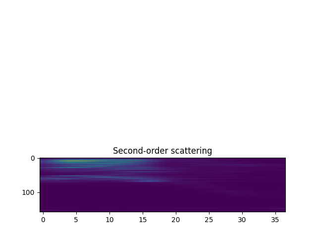
Finally, we plot the second-order scattering coefficients. These are also organized aling time, but has two log-frequency indices: one first-order frequency and one second-order frequency. Here, both indices are mixed along the vertical axis.

plt.subplot(3, 1, 3)
plt.imshow(Sx[order2], aspect='auto')
plt.title('Second-order scattering')

Text(0.5, 1.0, 'Second-order scattering')

Display the plots!

plt.tight_layout()
plt.show()