Plot the 1D wavelet filters

Let us examine the wavelet filters used by kymatio to calculate 1D scattering transforms. Filters are generated using the kymatio.scattering1d.filter_bank.scattering_filter_factory() method, which creates both the first- and second-order filter banks.

Preliminaries

from kymatio.scattering1d.filter_bank import scattering_filter_factory

We then import numpy and matplotlib to display the filters.

import numpy as np
import matplotlib.pyplot as plt

Filter parameters and generation

The filters are defined for a certain support size T which corresponds to the size of the input signal. The only restriction is that T must be a power of two. Since we are not computing any scattering transforms here, we may pick any power of two for T. Here, we choose 2**13 = 8192.

T = 2**13

The parameter J specifies the maximum scale of the low-pass filters as a power of two. In other words, the largest filter will be concentrated in a time interval of size 2**J.

J = 5

The Q parameter controls the number of wavelets per octave in the

first-and second-order filter banks. The larger the value, the narrower these filters in the frequency domain and the wider they are in the time domain (in general, the number of non-negligible oscillations in time is proportional to Q). For audio signals, it is often beneficial to have a large value for Q1 (between 4 and 16), since these signals are often highly oscillatory and

are better localized in frequency than they are in time. For the second layer,

Q2 is typically equal to 1 or 2. In this example, we set Q1=8 and Q2=1. Hence:

Q = (8, 1)

We are now ready to create the filters. These are generated by the scattering_filter_factory method, which takes the logarithm of T and the J and Q parameters. It returns the lowpass filter (phi_f), the first-order wavelet filters (psi1_f), and the second-order filters (psi2_f).

phi_f, psi1_f, psi2_f = scattering_filter_factory(T, J, Q, T)

The phi_f output is a dictionary where each integer key corresponds points to the instantiation of the filter at a certain resolution. Specifically, phi_f[‘levels’][0] corresponds to the lowpass filter at resolution T, while phi_f[‘levels’][1] corresponds to the filter at resolution T/2, and so on.

While phi_f only contains a single filter (at different resolutions), the psi1_f and psi2_f outputs are lists of filters, one for each wavelet bandpass filter in the filter bank.

Plot the frequency response of the filters

We are now ready to plot the frequency response of the filters. We first display the lowpass filter (at full resolution) in red. We then plot each of the bandpass filters in blue. Since we don’t care about the negative frequencies, we limit the plot to the frequency interval \([0, 0.5]\).

plt.figure()
plt.rcParams.update({"text.usetex": True})
plt.plot(np.arange(T)/T, phi_f['levels'][0], 'r')

for psi_f in psi1_f:
    plt.plot(np.arange(T)/T, psi_f['levels'][0], 'b')

plt.xlim(0, 0.5)

plt.xlabel(r'$\omega$', fontsize=18)
plt.ylabel(r'$\hat\psi_j(\omega)$', fontsize=18)
plt.title('Frequency response of first-order filters (Q = {})'.format(Q),
          fontsize=12)

Text(0.5, 1.0, 'Frequency response of first-order filters (Q = (8, 1))')

Do the same plot for the second-order filters. Note that since here Q = 1, we obtain wavelets that have higher frequency bandwidth.

plt.figure()
plt.rcParams.update({"text.usetex": True})
plt.plot(np.arange(T)/T, phi_f['levels'][0], 'r')
for psi_f in psi2_f:
    plt.plot(np.arange(T)/T, psi_f['levels'][0], 'b')
plt.xlim(0, 0.5)
plt.ylim(0, 1.2)
plt.xlabel(r'$\omega$', fontsize=18)
plt.ylabel(r'$\hat\psi_j(\omega)$', fontsize=18)
plt.title('Frequency response of second-order filters (Q = 1)', fontsize=12)

Text(0.5, 1.0, 'Frequency response of second-order filters (Q = 1)')

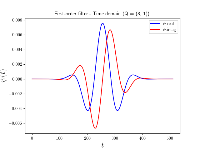
Plot the filter in time domain

The filters have been generated directly in the frequency domain to efficiently compute the convolution using the fft. By applying the ifft we get the filters in the time domain yielding analytic wavelets. We plot the first-order largest wavelet band-pass filter here.

plt.figure()
plt.rcParams.update({"text.usetex": True})

psi_time = np.fft.ifft(psi1_f[-1]['levels'][0])
psi_real = np.real(psi_time)
psi_imag = np.imag(psi_time)
plt.plot(np.concatenate((psi_real[-2**8:],psi_real[:2**8])),'b')
plt.plot(np.concatenate((psi_imag[-2**8:],psi_imag[:2**8])),'r')


plt.xlabel(r'$t$', fontsize=18)
plt.ylabel(r'$\psi(t)$', fontsize=18)
plt.title('First-order filter - Time domain (Q = {})'.format(Q), fontsize=12)
plt.legend(["$\psi$_real","$\psi$_imag"])

plt.show()