Classification of spoken digit recordings

In this example we use the 1D scattering transform to represent spoken digits, which we then classify using a simple classifier. This shows that 1D scattering representations are useful for this type of problem.

This dataset is automatically downloaded and preprocessed from https://github.com/Jakobovski/free-spoken-digit-dataset.git

Downloading and precomputing scattering coefficients should take about 5 min. Running the gradient descent takes about 1 min.

Results: Training accuracy = 99.7% Testing accuracy = 98.0%

Preliminaries

Since we’re using PyTorch to train the model, import torch.

import torch

We will be constructing a logistic regression classifier on top of the scattering coefficients, so we need some of the neural network tools from torch.nn and the Adam optimizer from torch.optim.

from torch.nn import Linear, NLLLoss, LogSoftmax, Sequential
from torch.optim import Adam

To handle audio file I/O, we import os and scipy.io.wavfile. We also need numpy for some basic array manipulation.

from scipy.io import wavfile
import os
import numpy as np

To evaluate our results, we need to form a confusion matrix using scikit-learn and display them using matplotlib.

from sklearn.metrics import confusion_matrix
import matplotlib.pyplot as plt

Finally, we import the Scattering1D class from the kymatio.torch package and the fetch_fsdd function from kymatio.datasets. The Scattering1D class is what lets us calculate the scattering transform, while the fetch_fsdd function downloads the FSDD, if needed.

from kymatio.torch import Scattering1D
from kymatio.datasets import fetch_fsdd

Pipeline setup

We start by specifying the dimensions of our processing pipeline along with some other parameters.

First, we have signal length. Longer signals are truncated and shorter signals are zero-padded. The sampling rate is 8000 Hz, so this corresponds to little over a second.

T = 2**13

Maximum scale 2**J of the scattering transform (here, about 30 milliseconds) and the number of wavelets per octave.

J = 8
Q = 12

We need a small constant to add to the scattering coefficients before computing the logarithm. This prevents very large values when the scattering coefficients are very close to zero.

log_eps = 1e-6

If a GPU is available, let’s use it!

use_cuda = torch.cuda.is_available()
device = torch.device("cuda" if use_cuda else "cpu")

For reproducibility, we fix the seed of the random number generator.

torch.manual_seed(42)

<torch._C.Generator object at 0x7f365969cf90>

Loading the data

Once the parameter are set, we can start loading the data into a format that can be fed into the scattering transform and then a logistic regression classifier.

We first download the dataset. If it’s already downloaded, fetch_fsdd will simply return the information corresponding to the dataset that’s already on disk.

info_data = fetch_fsdd()
files = info_data['files']
path_dataset = info_data['path_dataset']

Set up Tensors to hold the audio signals (x_all), the labels (y_all), and whether the signal is in the train or test set (subset).

x_all = torch.zeros(len(files), T, dtype=torch.float32, device=device)
y_all = torch.zeros(len(files), dtype=torch.int64, device=device)
subset = torch.zeros(len(files), dtype=torch.int64, device=device)

For each file in the dataset, we extract its label y and its index from the filename. If the index is between 0 and 4, it is placed in the test set, while files with larger indices are used for training. The actual signals are normalized to have maximum amplitude one, and are truncated or zero-padded to the desired length T. They are then stored in the x_all Tensor while their labels are in y_all.

for k, f in enumerate(files):
    basename = f.split('.')[0]

    # Get label (0-9) of recording.
    y = int(basename.split('_')[0])

    # Index larger than 5 gets assigned to training set.
    if int(basename.split('_')[2]) >= 5:
        subset[k] = 0
    else:
        subset[k] = 1

    # Load the audio signal and normalize it.
    _, x = wavfile.read(os.path.join(path_dataset, f))
    x = np.asarray(x, dtype='float')
    x /= np.max(np.abs(x))

    # Convert from NumPy array to PyTorch Tensor.
    x = torch.from_numpy(x).to(device)

    # If it's too long, truncate it.
    if x.numel() > T:
        x = x[:T]

    # If it's too short, zero-pad it.
    start = (T - x.numel()) // 2

    x_all[k,start:start + x.numel()] = x
    y_all[k] = y

Log-scattering transform

We now create the Scattering1D object that will be used to calculate the scattering coefficients.

scattering = Scattering1D(J, T, Q).to(device)

Compute the scattering transform for all signals in the dataset.

Sx_all = scattering.forward(x_all)

Since it does not carry useful information, we remove the zeroth-order scattering coefficients, which are always placed in the first channel of the scattering Tensor.

Sx_all = Sx_all[:,1:,:]

To increase discriminability, we take the logarithm of the scattering coefficients (after adding a small constant to make sure nothing blows up when scattering coefficients are close to zero). This is known as the log-scattering transform.

Sx_all = torch.log(torch.abs(Sx_all) + log_eps)

Finally, we average along the last dimension (time) to get a time-shift invariant representation.

Sx_all = torch.mean(Sx_all, dim=-1)

Training the classifier

With the log-scattering coefficients in hand, we are ready to train our logistic regression classifier.

First, we extract the training data (those for which subset equals 0) and the associated labels.

Sx_tr, y_tr = Sx_all[subset == 0], y_all[subset == 0]

Standardize the data to have mean zero and unit variance. Note that we need to apply the same transformation to the test data later, so we save the mean and standard deviation Tensors.

mu_tr = Sx_tr.mean(dim=0)
std_tr = Sx_tr.std(dim=0)
Sx_tr = (Sx_tr - mu_tr) / std_tr

Here we define a logistic regression model using PyTorch. We train it using Adam with a negative log-likelihood loss.

num_input = Sx_tr.shape[-1]
num_classes = y_tr.cpu().unique().numel()
model = Sequential(Linear(num_input, num_classes), LogSoftmax(dim=1))
optimizer = Adam(model.parameters())
criterion = NLLLoss()

If we’re on a GPU, transfer the model and the loss function onto the device.

model = model.to(device)
criterion = criterion.to(device)

Before training the model, we set some parameters for the optimization procedure.

# Number of signals to use in each gradient descent step (batch).
batch_size = 32
# Number of epochs.
num_epochs = 50
# Learning rate for Adam.
lr = 1e-4

Given these parameters, we compute the total number of batches.

nsamples = Sx_tr.shape[0]
nbatches = nsamples // batch_size

Now we’re ready to train the classifier.

for e in range(num_epochs):
    # Randomly permute the data. If necessary, transfer the permutation to the
    # GPU.
    perm = torch.randperm(nsamples, device=device)

    # For each batch, calculate the gradient with respect to the loss and take
    # one step.
    for i in range(nbatches):
        idx = perm[i * batch_size : (i+1) * batch_size]
        model.zero_grad()
        resp = model.forward(Sx_tr[idx])
        loss = criterion(resp, y_tr[idx])
        loss.backward()
        optimizer.step()

    # Calculate the response of the training data at the end of this epoch and
    # the average loss.
    resp = model.forward(Sx_tr)
    avg_loss = criterion(resp, y_tr)

    # Try predicting the classes of the signals in the training set and compute
    # the accuracy.
    y_hat = resp.argmax(dim=1)
    accuracy = (y_tr == y_hat).float().mean()

    print('Epoch {}, average loss = {:1.3f}, accuracy = {:1.3f}'.format(
        e, avg_loss, accuracy))

Epoch 0, average loss = 0.727, accuracy = 0.816
Epoch 1, average loss = 0.508, accuracy = 0.879
Epoch 2, average loss = 0.407, accuracy = 0.909
Epoch 3, average loss = 0.347, accuracy = 0.919
Epoch 4, average loss = 0.308, accuracy = 0.927
Epoch 5, average loss = 0.280, accuracy = 0.938
Epoch 6, average loss = 0.256, accuracy = 0.942
Epoch 7, average loss = 0.236, accuracy = 0.947
Epoch 8, average loss = 0.219, accuracy = 0.950
Epoch 9, average loss = 0.207, accuracy = 0.952
Epoch 10, average loss = 0.197, accuracy = 0.953
Epoch 11, average loss = 0.185, accuracy = 0.956
Epoch 12, average loss = 0.178, accuracy = 0.959
Epoch 13, average loss = 0.165, accuracy = 0.962
Epoch 14, average loss = 0.160, accuracy = 0.961
Epoch 15, average loss = 0.152, accuracy = 0.965
Epoch 16, average loss = 0.148, accuracy = 0.964
Epoch 17, average loss = 0.141, accuracy = 0.970
Epoch 18, average loss = 0.137, accuracy = 0.970
Epoch 19, average loss = 0.131, accuracy = 0.971
Epoch 20, average loss = 0.127, accuracy = 0.973
Epoch 21, average loss = 0.122, accuracy = 0.977
Epoch 22, average loss = 0.119, accuracy = 0.974
Epoch 23, average loss = 0.115, accuracy = 0.978
Epoch 24, average loss = 0.113, accuracy = 0.973
Epoch 25, average loss = 0.109, accuracy = 0.977
Epoch 26, average loss = 0.104, accuracy = 0.980
Epoch 27, average loss = 0.106, accuracy = 0.981
Epoch 28, average loss = 0.107, accuracy = 0.976
Epoch 29, average loss = 0.098, accuracy = 0.980
Epoch 30, average loss = 0.094, accuracy = 0.983
Epoch 31, average loss = 0.093, accuracy = 0.981
Epoch 32, average loss = 0.094, accuracy = 0.979
Epoch 33, average loss = 0.091, accuracy = 0.983
Epoch 34, average loss = 0.086, accuracy = 0.983
Epoch 35, average loss = 0.085, accuracy = 0.985
Epoch 36, average loss = 0.082, accuracy = 0.983
Epoch 37, average loss = 0.081, accuracy = 0.986
Epoch 38, average loss = 0.077, accuracy = 0.987
Epoch 39, average loss = 0.077, accuracy = 0.984
Epoch 40, average loss = 0.074, accuracy = 0.987
Epoch 41, average loss = 0.072, accuracy = 0.988
Epoch 42, average loss = 0.072, accuracy = 0.989
Epoch 43, average loss = 0.071, accuracy = 0.989
Epoch 44, average loss = 0.070, accuracy = 0.987
Epoch 45, average loss = 0.068, accuracy = 0.989
Epoch 46, average loss = 0.066, accuracy = 0.987
Epoch 47, average loss = 0.065, accuracy = 0.991
Epoch 48, average loss = 0.064, accuracy = 0.989
Epoch 49, average loss = 0.062, accuracy = 0.991

Now that our network is trained, let’s test it!

First, we extract the test data (those for which subset equals 1) and the associated labels.

Sx_te, y_te = Sx_all[subset == 1], y_all[subset == 1]

Use the mean and standard deviation calculated on the training data to standardize the testing data, as well.

Sx_te = (Sx_te - mu_tr) / std_tr

Calculate the response of the classifier on the test data and the resulting loss.

resp = model.forward(Sx_te)
avg_loss = criterion(resp, y_te)

# Try predicting the labels of the signals in the test data and compute the
# accuracy.

y_hat = resp.argmax(dim=1)
accu = (y_te == y_hat).float().mean()

print('TEST, average loss = {:1.3f}, accuracy = {:1.3f}'.format(
      avg_loss, accu))

TEST, average loss = 0.110, accuracy = 0.967

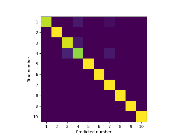
Plotting the classification accuracy as a confusion matrix

Let’s see what the very few misclassified sounds get misclassified as. We will plot a confusion matrix which indicates in a 2D histogram how often one sample was mistaken for another (anything on the diagonal is correctly classified, anything off the diagonal is wrong).

predicted_categories = y_hat.cpu().numpy()
actual_categories = y_te.cpu().numpy()

confusion = confusion_matrix(actual_categories, predicted_categories)
plt.figure()
plt.imshow(confusion)
tick_locs = np.arange(10)
ticks = ['{}'.format(i) for i in range(1, 11)]
plt.xticks(tick_locs, ticks)
plt.yticks(tick_locs, ticks)
plt.ylabel("True number")
plt.xlabel("Predicted number")
plt.show()