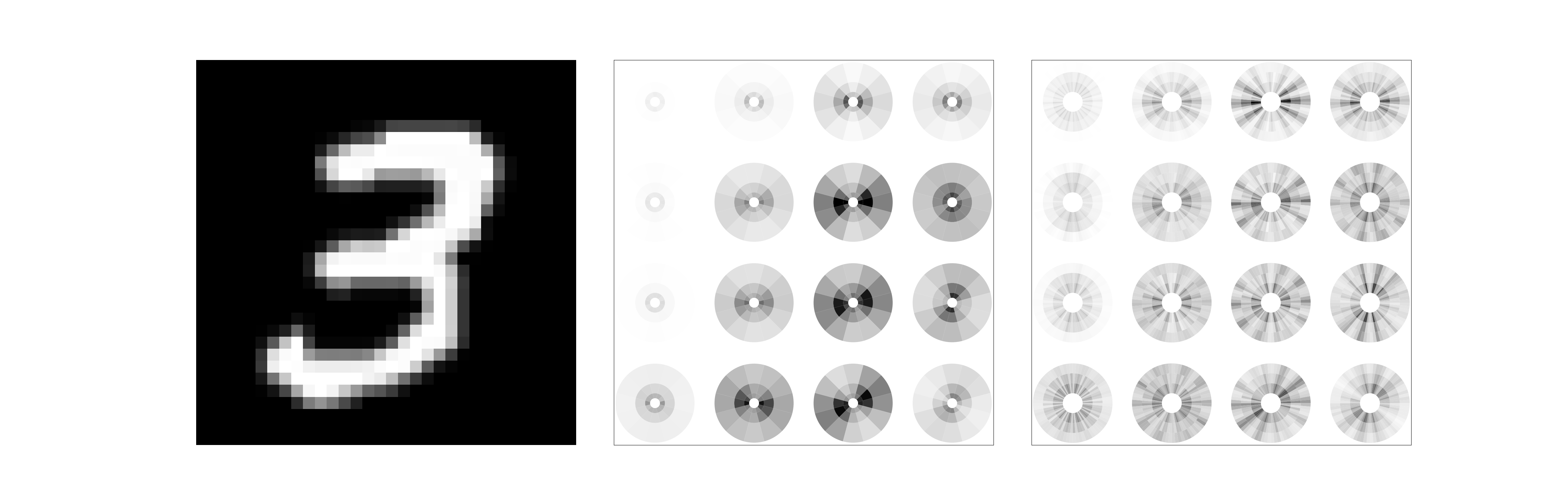
Scattering disk display

This script reproduces the display of scattering coefficients amplitude within a disk as described in “Invariant Scattering Convolution Networks” by J. Bruna and S. Mallat (2012) (https://arxiv.org/pdf/1203.1513.pdf).

Author: https://github.com/Jonas1312

Edited by: Edouard Oyallon and anakin-datawalker

import matplotlib as mpl
import matplotlib.cm as cm
import matplotlib.pyplot as plt
from matplotlib import gridspec
import numpy as np
from kymatio import Scattering2D
from PIL import Image
import os

img_name = os.path.join(os.getcwd(), "images/digit.png")

Scattering computations

First, we read the input digit:

src_img = Image.open(img_name).convert('L').resize((32, 32))
src_img = np.array(src_img)
print("img shape: ", src_img.shape)

img shape:  (32, 32)

We compute a Scattering Transform with \(L=6\) angles and \(J=3\) scales.

Morlet wavelets \(\psi_{\theta}\) are Hermitian, i.e: \(\psi_{\theta}^*(u) = \psi_{\theta}(-u) = \psi_{\theta+\pi}(u)\).

As a consequence, the modulus wavelet transform of a real signal \(x\) computed with a Morlet wavelet \(\psi_{\theta}\) is invariant by a rotation of \(\pi\) of the wavelet. Indeed, since \((x*\psi_{\theta}(u))^* = x*(\psi_{\theta}^*)(u) = x*\psi_{\theta+\pi}(u)\), we have \(\lvert x*\psi_{\theta}(u)\rvert = \lvert x*\psi_{\theta+\pi}(u)\rvert\).

Scattering coefficients of order \(n\): \(\lvert \lvert \lvert x * \psi_{\theta_1, j_1} \rvert * \psi_{\theta_2, j_2} \rvert \cdots * \psi_{\theta_n, j_n} \rvert * \phi_J\) are thus invariant to a rotation of \(\pi\) of any wavelet \(\psi_{\theta_i, j_i}\). As a consequence, Kymatio computes scattering coefficients with \(L\) wavelets whose orientation is uniformly sampled in an interval of length \(\pi\).

L = 6
J = 3
scattering = Scattering2D(J=J, shape=src_img.shape, L=L, max_order=2, frontend='numpy')

We now compute the scattering coefficients:

src_img_tensor = src_img.astype(np.float32) / 255.

scat_coeffs = scattering(src_img_tensor)
print("coeffs shape: ", scat_coeffs.shape)
# Invert colors
scat_coeffs= -scat_coeffs

coeffs shape:  (127, 4, 4)

There are 127 scattering coefficients, among which 1 is low-pass, \(JL=18\) are of first-order and \(L^2(J(J-1)/2)=108\) are of second-order. Due to the subsampling by \(2^J=8\), the final spatial grid is of size \(4\times4\). We now retrieve first-order and second-order coefficients for the display.

len_order_1 = J*L
scat_coeffs_order_1 = scat_coeffs[1:1+len_order_1, :, :]
norm_order_1 = mpl.colors.Normalize(scat_coeffs_order_1.min(), scat_coeffs_order_1.max(), clip=True)
mapper_order_1 = cm.ScalarMappable(norm=norm_order_1, cmap="gray")
# Mapper of coefficient amplitude to a grayscale color for visualisation.

len_order_2 = (J*(J-1)//2)*(L**2)
scat_coeffs_order_2 = scat_coeffs[1+len_order_1:, :, :]
norm_order_2 = mpl.colors.Normalize(scat_coeffs_order_2.min(), scat_coeffs_order_2.max(), clip=True)
mapper_order_2 = cm.ScalarMappable(norm=norm_order_2, cmap="gray")
# Mapper of coefficient amplitude to a grayscale color for visualisation.

# Retrieve spatial size
window_rows, window_columns = scat_coeffs.shape[1:]
print("nb of (order 1, order 2) coefficients: ", (len_order_1, len_order_2))

nb of (order 1, order 2) coefficients:  (18, 108)

Figure reproduction

Now we can reproduce a figure that displays the amplitude of first-order and second-order scattering coefficients within a disk like in Bruna and Mallat’s paper.

For visualisation purposes, we display first-order scattering coefficients \(\lvert x * \psi_{\theta_1, j_1} \rvert * \phi_J\) with \(2L\) angles \(\theta_1\) spanning \([0,2\pi]\) using the central symmetry of those coefficients explained above. We similarly display second-order scattering coefficients \(\lvert \lvert x * \psi_{\theta_1, j_1} \rvert * \psi_{\theta_2, j_2} \rvert * \phi_J\) with \(2L\) angles \(\theta_1\) spanning \([0,2\pi]\) but keep only \(L\) orientations for \(\theta_2\) (and thus an interval of \(\pi\)), so as not to overload the display.

Here, each scattering coefficient is represented on the polar plane within a quadrant indexed by a radius and an angle.

For first-order coefficients, the polar radius is inversely proportional to the scale \(2^{j_1}\) of the wavelet \(\psi_{\theta_1, j_1}\) while the angle corresponds to the orientation \(\theta_1\). The surface of each quadrant is also inversely proportional to the scale \(2^{j_1}\), which corresponds to the frequency bandwidth of the Fourier transform \(\hat{\psi}_{\theta_1, j_1}\). First-order scattering quadrants can thus be indexed by \((\theta_1,j_1)\).

For second-order coefficients, each first-order quadrant is equally divided along the radius axis by the number of increasing scales \(j_1 < j_2 < J\) and by \(L\) along the angle axis to produce a quadrant indexed by \((\theta_1,\theta_2, j_1, j_2)\). It simply means in our case where \(J=3\) that the first-order quadrant corresponding to \(j_1=0\) is subdivided along its radius in 2 equal quadrants corresponding to \(j_2 \in \{1,2\}\), which are each further divided by the \(L\) possible \(\theta_2\) angles, and that \(j_1=1\) quadrants are only divided by \(L\), corresponding to \(j_2=2\) and the \(L\) possible \(\theta_2\). Note that no second-order coefficients are thus associated to \(j_1=2\) in this case whose quadrants are just left blank.

Observe how the amplitude of first-order coefficients is strongest along the direction of edges, and that they exhibit by construction a central symmetry.

# Define figure size and grid on which to plot input digit image, first-order and second-order scattering coefficients
fig = plt.figure(figsize=(47, 15))
spec = fig.add_gridspec(ncols=3, nrows=1)

gs = gridspec.GridSpec(1, 3, wspace=0.1)
gs_order_1 = gridspec.GridSpecFromSubplotSpec(window_rows, window_columns, subplot_spec=gs[1])
gs_order_2 = gridspec.GridSpecFromSubplotSpec(window_rows, window_columns, subplot_spec=gs[2])

# Start by plotting input digit image and invert colors
ax = plt.subplot(gs[0])
ax.set_xticks([])
ax.set_yticks([])
ax.imshow(src_img,cmap='gray',interpolation='nearest', aspect='auto')
ax.axis('off')

# Plot first-order scattering coefficients
ax = plt.subplot(gs[1])
ax.set_xticks([])
ax.set_yticks([])

l_offset = int(L - L / 2 - 1)  # follow same ordering as Kymatio for angles

for row in range(window_rows):
    for column in range(window_columns):
        ax = fig.add_subplot(gs_order_1[row, column], projection='polar')
        ax.axis('off')
        coefficients = scat_coeffs_order_1[:, row, column]
        for j in range(J):
            for l in range(L):
                coeff = coefficients[l + j * L]
                color = mapper_order_1.to_rgba(coeff)
                angle = (l_offset - l) * np.pi / L
                radius = 2 ** (-j - 1)
                ax.bar(x=angle,
                       height=radius,
                       width=np.pi / L,
                       bottom=radius,
                       color=color)
                ax.bar(x=angle + np.pi,
                       height=radius,
                       width=np.pi / L,
                       bottom=radius,
                       color=color)

# Plot second-order scattering coefficients
ax = plt.subplot(gs[2])
ax.set_xticks([])
ax.set_yticks([])

for row in range(window_rows):
    for column in range(window_columns):
        ax = fig.add_subplot(gs_order_2[row, column], projection='polar')
        ax.axis('off')
        coefficients = scat_coeffs_order_2[:, row, column]
        for j1 in range(J - 1):
            for j2 in range(j1 + 1, J):
                for l1 in range(L):
                    for l2 in range(L):
                        coeff_index = l1 * L * (J - j1 - 1) + l2 + L * (j2 - j1 - 1) + (L ** 2) * \
                                      (j1 * (J - 1) - j1 * (j1 - 1) // 2)
                        # indexing a bit complex which follows the order used by Kymatio to compute
                        # scattering coefficients
                        coeff = coefficients[coeff_index]
                        color = mapper_order_2.to_rgba(coeff)
                        # split along angles first-order quadrants in L quadrants, using same ordering
                        # as Kymatio (clockwise) and center (with the 0.5 offset)
                        angle = (l_offset - l1) * np.pi / L + (L // 2 - l2 - 0.5) * np.pi / (L ** 2)
                        radius = 2 ** (-j1 - 1)
                        # equal split along radius is performed through height variable
                        ax.bar(x=angle,
                               height=radius / 2 ** (J - 2 - j1),
                               width=np.pi / L ** 2,
                               bottom=radius + (radius / 2 ** (J - 2 - j1)) * (J - j2 - 1),
                               color=color)
                        ax.bar(x=angle + np.pi,
                               height=radius / 2 ** (J - 2 - j1),
                               width=np.pi / L ** 2,
                               bottom=radius + (radius / 2 ** (J - 2 - j1)) * (J - j2 - 1),
                               color=color)