Plot the 2D wavelet filters¶

See kymatio.scattering2d.filter_bank() for more informations about the used wavelets.

from colorsys import hls_to_rgb
import matplotlib.pyplot as plt
import numpy as np
from kymatio.scattering2d.filter_bank import filter_bank
from scipy.fft import fft2

Initial parameters of the filter bank¶

M = 32
J = 3
L = 8
filters_set = filter_bank(M, M, J, L=L)

Imshow complex images¶

Thanks to https://stackoverflow.com/questions/17044052/mathplotlib-imshow-complex-2d-array

def colorize(z):
    n, m = z.shape
    c = np.zeros((n, m, 3))
    c[np.isinf(z)] = (1.0, 1.0, 1.0)
    c[np.isnan(z)] = (0.5, 0.5, 0.5)

    idx = ~(np.isinf(z) + np.isnan(z))
    A = (np.angle(z[idx]) + np.pi) / (2*np.pi)
    A = (A + 0.5) % 1.0
    B = 1.0/(1.0 + abs(z[idx])**0.3)
    c[idx] = [hls_to_rgb(a, b, 0.8) for a, b in zip(A, B)]
    return c

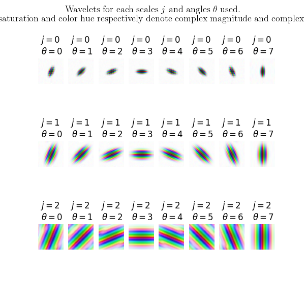
Bandpass filters¶

First, we display each wavelet according to its scale and orientation.

fig, axs = plt.subplots(J, L, sharex=True, sharey=True)
fig.set_figheight(6)
fig.set_figwidth(6)
plt.rc('text', usetex=True)
plt.rc('font', family='serif')
i = 0
for filter in filters_set['psi']:
    f = filter["levels"][0]
    filter_c = fft2(f)
    filter_c = np.fft.fftshift(filter_c)
    axs[i // L, i % L].imshow(colorize(filter_c))
    axs[i // L, i % L].axis('off')
    axs[i // L, i % L].set_title(
        "$j = {}$ \n $\\theta={}$".format(i // L, i % L))
    i = i+1

fig.suptitle((r"Wavelets for each scales $j$ and angles $\theta$ used."
              "\nColor saturation and color hue respectively denote complex "
              "magnitude and complex phase."), fontsize=13)
fig.show()

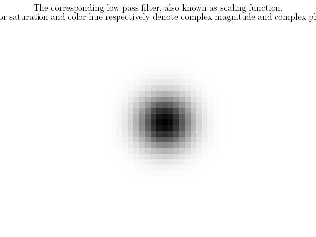
$Wavelets for each scales $j$ and angles $\theta$ used. Color saturation and color hue respectively denote complex magnitude and complex phase., $j = 0$ $\theta=0$, $j = 0$ $\theta=1$, $j = 0$ $\theta=2$, $j = 0$ $\theta=3$, $j = 0$ $\theta=4$, $j = 0$ $\theta=5$, $j = 0$ $\theta=6$, $j = 0$ $\theta=7$, $j = 1$ $\theta=0$, $j = 1$ $\theta=1$, $j = 1$ $\theta=2$, $j = 1$ $\theta=3$, $j = 1$ $\theta=4$, $j = 1$ $\theta=5$, $j = 1$ $\theta=6$, $j = 1$ $\theta=7$, $j = 2$ $\theta=0$, $j = 2$ $\theta=1$, $j = 2$ $\theta=2$, $j = 2$ $\theta=3$, $j = 2$ $\theta=4$, $j = 2$ $\theta=5$, $j = 2$ $\theta=6$, $j = 2$ $\theta=7$$

Lowpass filter¶

We finally display the low-pass filter.

plt.figure()
plt.rc('text', usetex=True)
plt.rc('font', family='serif')
plt.axis('off')
plt.set_cmap('gray_r')

f = filters_set['phi']["levels"][0]

filter_c = fft2(f)
filter_c = np.fft.fftshift(filter_c)
plt.suptitle(("The corresponding low-pass filter, also known as scaling "
              "function.\nColor saturation and color hue respectively denote "
              "complex magnitude and complex phase"), fontsize=13)
filter_c = np.abs(filter_c)
plt.imshow(filter_c)

plt.show()